In a previous post, I shared a simple modeling tool created using HTML, JavaScript, and CSS. The tool visualized the expected RSSI of a transmitter, utilizing variables such as frequency, TX power, distance, and height. However, the model assumed a transmitter and receiver gain of 0 dBm, which doesn’t reflect real-world conditions.
Typically, vendors provide radiation patterns in the form of elevation and azimuth diagrams. Unfortunately, these are often low-resolution images and not programmatically usable. This lack of structured data presents challenges for custom modeling efforts.
On the other hand, commercial tools like Ekahau, Hamina, AirMagnet, and iBwave integrate antennas with reliable accuracy. These tools likely receive detailed and structured data directly from vendors, allowing for precise modeling.
Without aiming to create a highly accurate model, I explored a method to extract antenna gain data directly from a modeling tool’s interface. Since I have access to Ekahau, I chose it as my platform for experimentation.
Methodology: Extracting Antenna Gain Data
After some consideration and trials, I developed the following approach:
- Create a Floorplan
Set up a floorplan to establish an accurate scale. - Configure Access Point Settings
Position the access point (AP) at a height of 1 meter (the same height as the client device) and configure the transmission power to 100 mW (though any value could be used). - Define a Measurement Radius
Place the AP and calculate the Free Space Path Loss (FSPL) for a given radius. I chose 100 meters to minimize small variations caused by pixel inaccuracies. - Collect Measurements
Measure signal strength at specific points along the defined radius. - Calculate Antenna Gain
Use the gathered data to calculate the gain at each measured point.
Automating Measurements
The primary challenge was automating the measurement process. To address this, I used the Python library pyautogui to simulate clicks every 5 degrees along the defined radius. Each click displayed the RSSI value at the corresponding angle.
To extract the RSSI data, the script captured screenshots of the RSSI display area and processed them using the OCR library pytesseract, which converted pixel data into text.
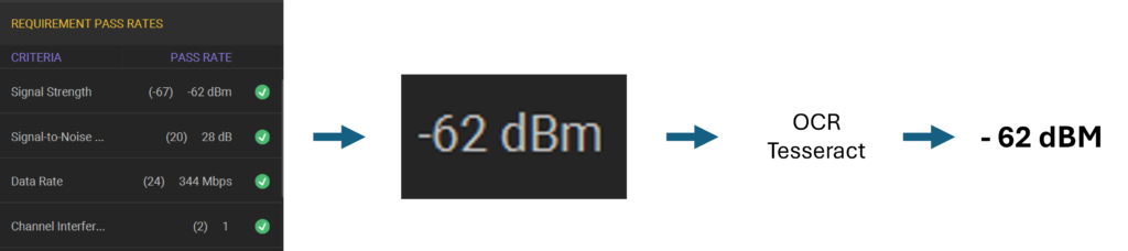
The final output was a CSV file containing three columns: angle, RSSI, and gain.
Calculating Antenna Gain
To calculate the gain of the transmitter, we can use the Friis Transmission Equation
Pr = Pt + Gt + Gr – Lf
Where:
- Pr : Received power in dBm (it is what is measured from Ekahau)
- Pt : Transmitted power in dBm (fixed 100mW = 20dBm)
- Gt : Transmitter gain in dBi (to be calculated)
- Gr : Receiver gain in dBi (considering 0 dBi)
- Lf : Free space path Loss (FSPL) in dB
FSPL(dB)=20log10(d)+20log10(f)+20log10(c4π)
Where:
- c : speed of light (299,792,458m/s )
- f : frequency in Hz
- d : distance in meters (fixed 100 meters)
For an isotropic antenna we have:
Pr_iso = Pt – Lf
Gain is:
Gt = Pr – Pr_iso
Pr is measured
Pr_iso is calculdated using Pt – Lf
Lf (FSPL) for 2.4 GHz is:
Lf = 20log10(100)+20log10(2412000000)+20log10(c4π) = -80.09 dB
Pr_iso = 20 dBm – 80.09 dB = -60.09 dBm
Lets say that I have measured -58dBm
Gt = -58dBm + 60.09dBm
Gt = 2,09 dBi
Btw -58 dBm was measured using a 2.2 dBi antenna.
Results
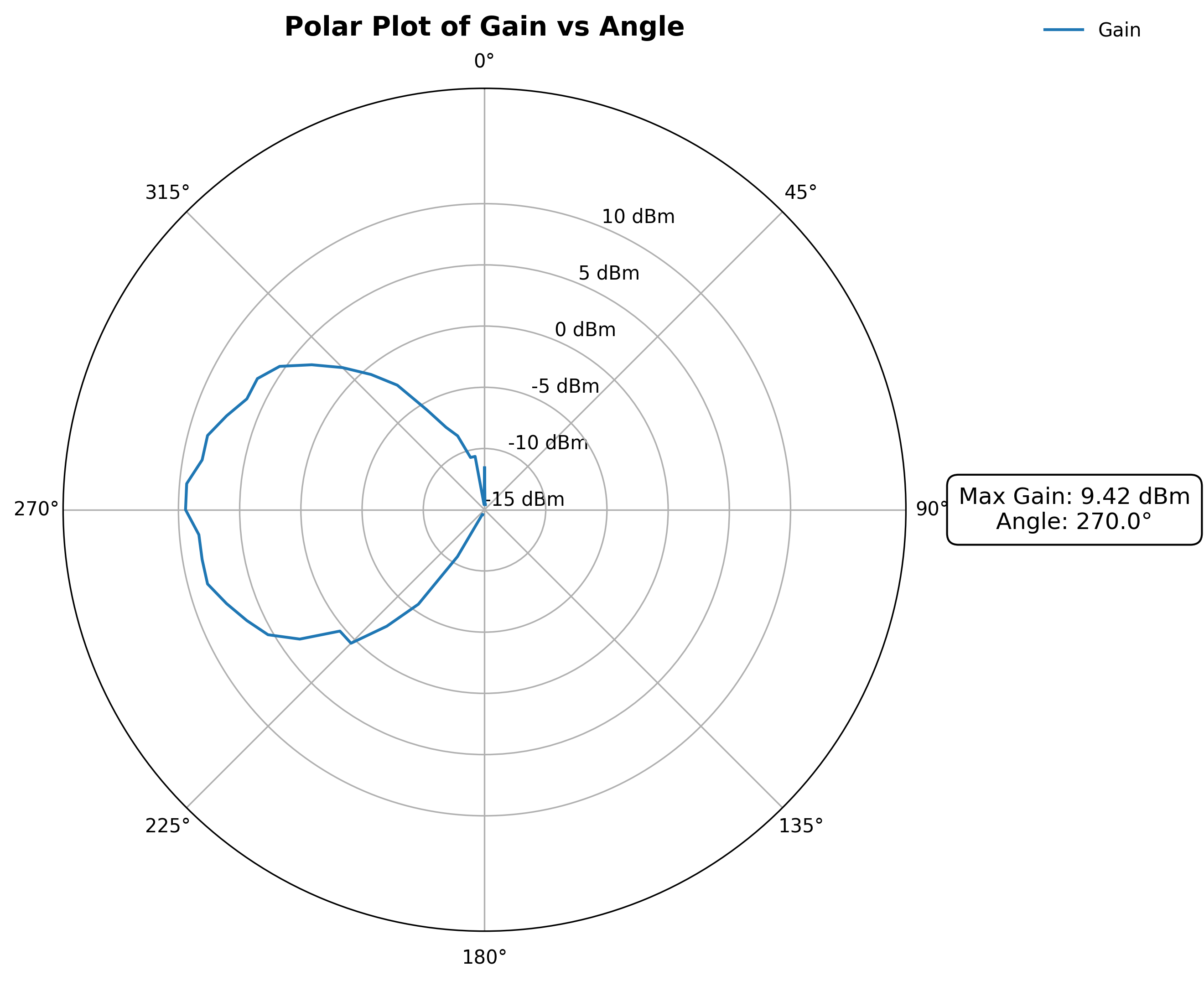
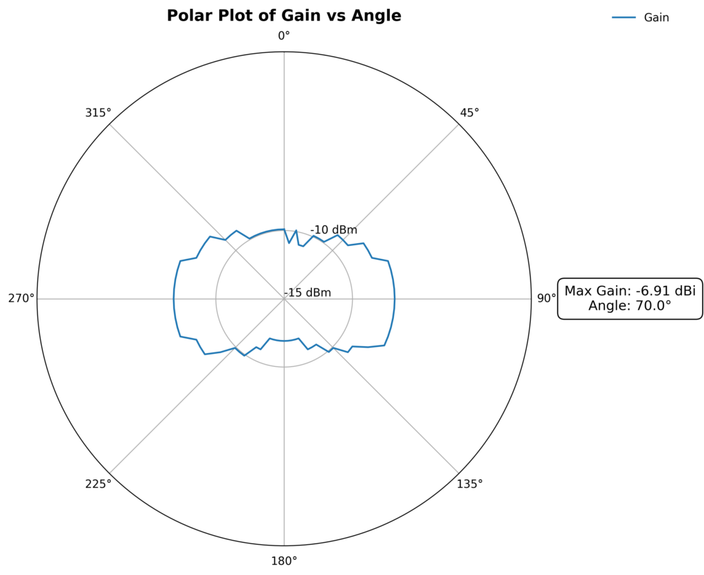
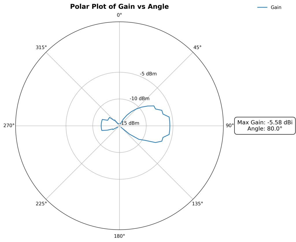
Using this method, I generated polar diagrams for various antennas, which visually represent their radiation patterns. Below is an example of the polar diagram generated for different antennas.
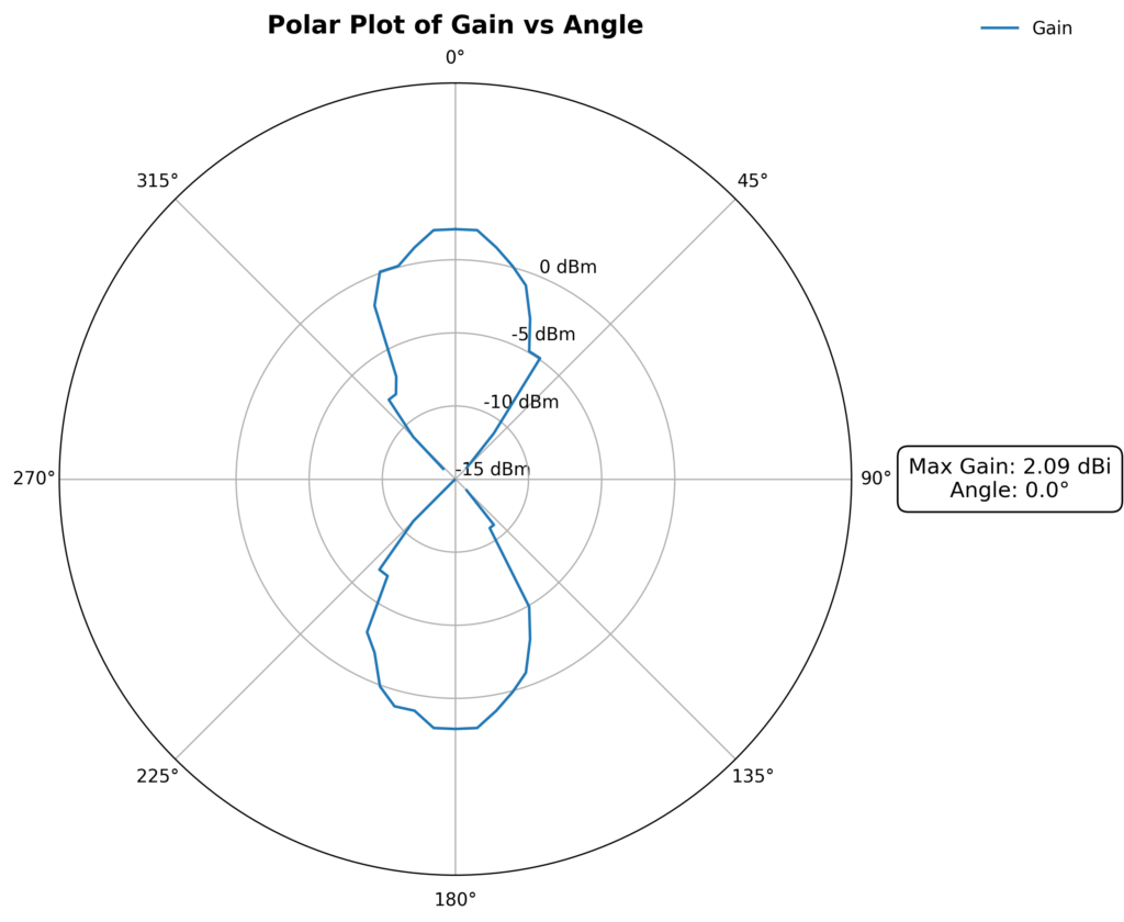
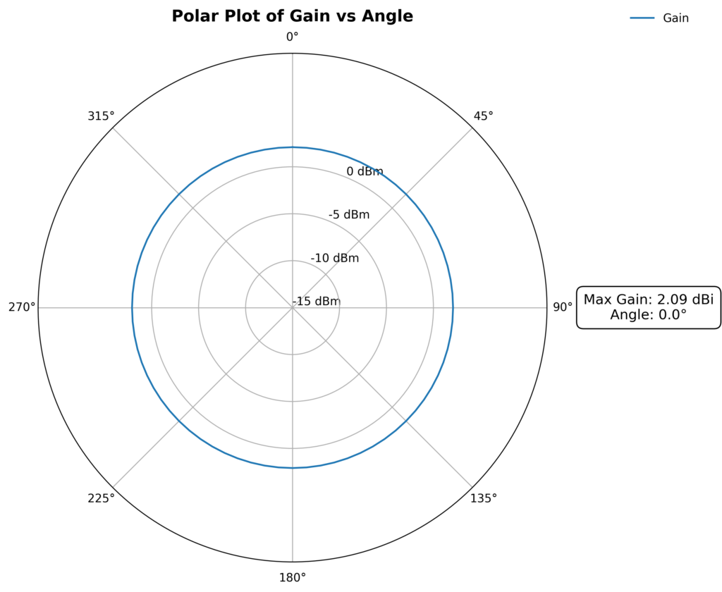
Using a generic Wi-Fi 6 device with a 2.2dBi omni antenna I got the max gain of 2.09 dBi. I tried to identify the reason of not getting the exact 2.2 dBi but could not figure it out.
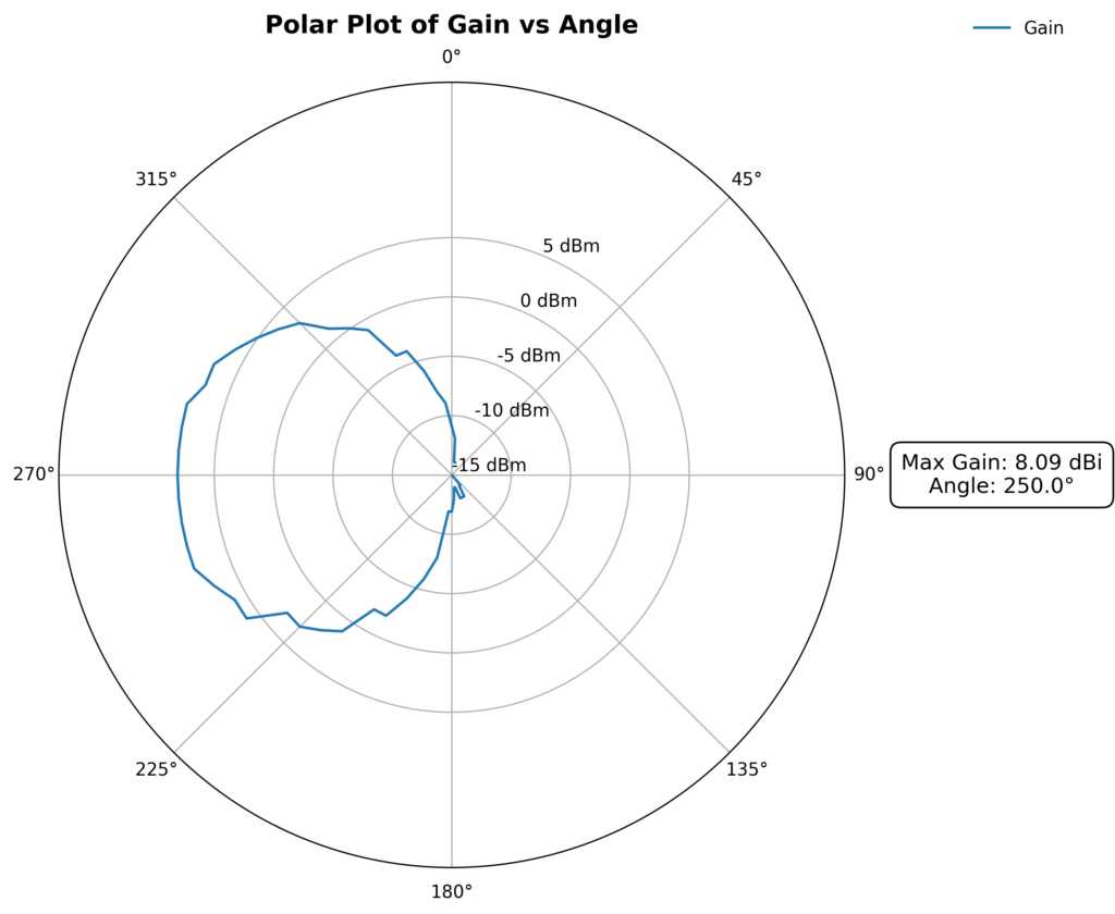
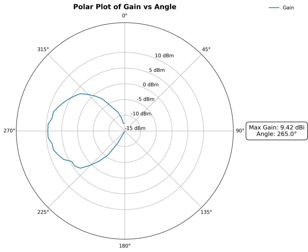
Doing the same process with the Cisco 1562D (2.4 GHz), I got a max calculated gain of 8.09 dBi, compared to the datasheet value of 9 dBi. For 5 GHz, the max calculated gain was 9.42 dBi, while the datasheet lists it as 10 dBi.
I couldn’t match the exact values—maybe the 5-degree steps weren’t precise enough.
For now, I’ll stick with these values. In the future, it won’t be hard to tweak the procedure to include whatever might be missing.
In the next post, I’ll integrate this data into the simulation tool, factoring in not just FSPL but also the transmitter gain.
Thanks,
Diego Capassi