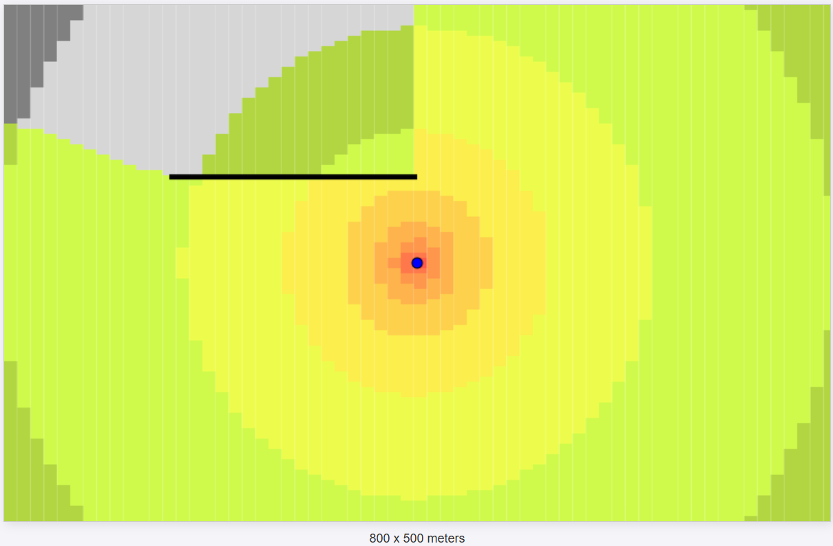
In the previous post, I shared a simple wireless propagation tool. Feel free to check it out if you haven’t already. In this post, we’ll add basic walls to the simulation, introducing loss into the system.

Please note that this is a simple simulation designed solely for study purposes.

When an RF signal passes through a wall, part of its energy is absorbed by the wall and converted into heat. Some of the signal—often a portion, but not always the majority—may be reflected, while the remaining energy passes through the wall with reduced strength, depending on the material’s properties and the signal’s frequency.

The goal is to incorporate the attenuation the signal experiences when passing through the walls.

The basic steps to add this feature to the simulation are:

1. Draw a basic wall using two points.
2. For each grid point, create a line segment to the transmitter.
3. Check if the segment crosses the wall.
4. Add the loss to the Friis Equation.

I’ve created a Wall class that includes two points and a wallType attribute. This allows us to simulate different material types.

To simplify visualization, we’ll start with a 10×10 block grid.

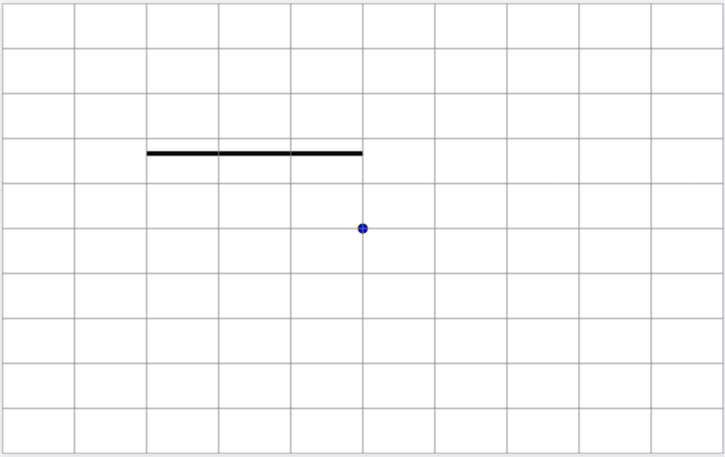
Each block checks whether the line segment from its center to the transmitter intersects with the wall.

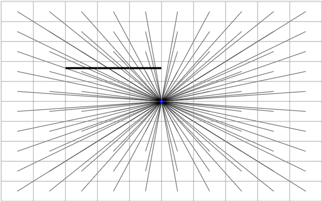
How can we determine if the line segment intersects the wall?

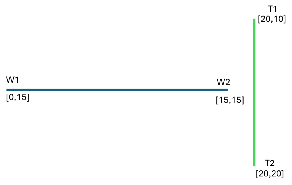
To simplify the process, let’s focus on a scenario below:

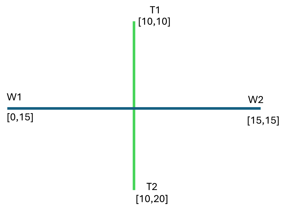
The idea is to check if W1 and W2 are on opposite sides relative to T1 and T2.

1. Create a vector “T” using the points T2 and T1:
   Vector_T = T2 – T1 = [0, 10]
2. Create a vector “W” using the points W2 and W1:
   Vector_W = W2 – W1 = [15, 0]
3. Create vectors from T1 to each wall point:
   • Vector_T1_W1 = W1 – T1 = [-10, 5]
   • Vector_T1_W2 = W2 – T1 = [5, 5]
4. Create vectors from W1 to T1 and T2:
   • Vector_W1_T1 = T1 – W1 = [10, -5]
   • Vector_W1_T2 = T2 – W1 = [10, 5]

Now, let’s plot these vectors to visualize the relationships.

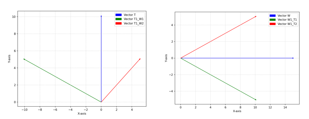
The vectors T and W are positioned between the other vectors, which indicates that the segments formed by W and T are crossing.

Using the cross product, we can determine the relationship between two vectors. The cross product shows whether the vectors are collinear, clockwise, or counterclockwise, depending on the sign.

The formula for the cross product is:
crossproduct(VectorA, VectorB) = (VectorA.x multiplied by VectorB.y) minus (VectorB.x multiplied by VectorA.y).

Cross product calculations for this case are as follows:

• c1 is the cross product of Vector T and Vector from T1 to W1, which equals -75.
• c2 is the cross product of Vector T and Vector from T1 to W2, which equals 75.
• c3 is the cross product of Vector W and Vector from W1 to T1, which equals 100.
• c4 is the cross product of Vector W and Vector from W1 to T2, which equals -50.

For the segments to cross, the condition is that the product of c1 and c2 is less than zero, and the product of c3 and c4 is also less than zero. This means that the sign of each pair must be opposite.

In this case, the condition is satisfied, meaning the segments do intersect.

Now, let us apply the same procedure to the next scenario:

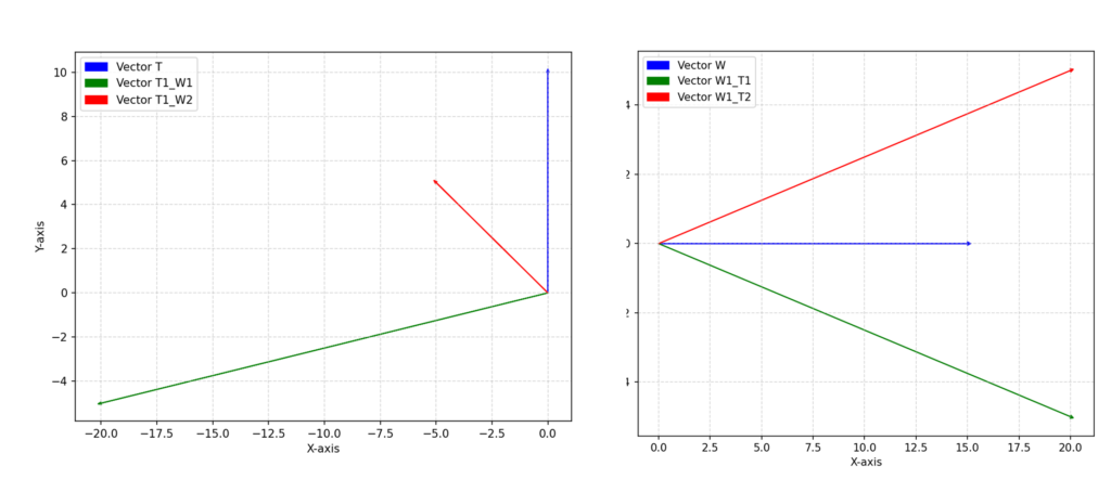
We can see that Vector T has the vectors from T1 to W1 and from T1 to W2 in the same orientation (counterclockwise), which is enough to conclude that the segments do not intersect.

The cross product results are:

• The cross product of Vector T and Vector from T1 to W1 is 2000.
• The cross product of Vector T and Vector from T1 to W2 is 50.
  (Both have the same orientation—counterclockwise.)
• The cross product of Vector W and Vector from W1 to T1 is -75.
• The cross product of Vector W and Vector from W1 to T2 is 75.

These results show that the segments do not intersect.

There is a special case where the segments could be collinear, but we will not discuss that here.

Next, we will implement this check for each block and plot whether the block has a crossing line to the transmitter, marking it as either “True” or “False.”

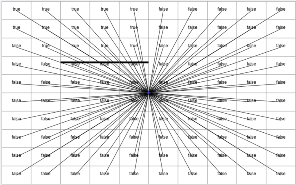
If the block where the signal is measured has a line segment to the transmitter that crosses a wall, the wall loss is added to the Friis equation.

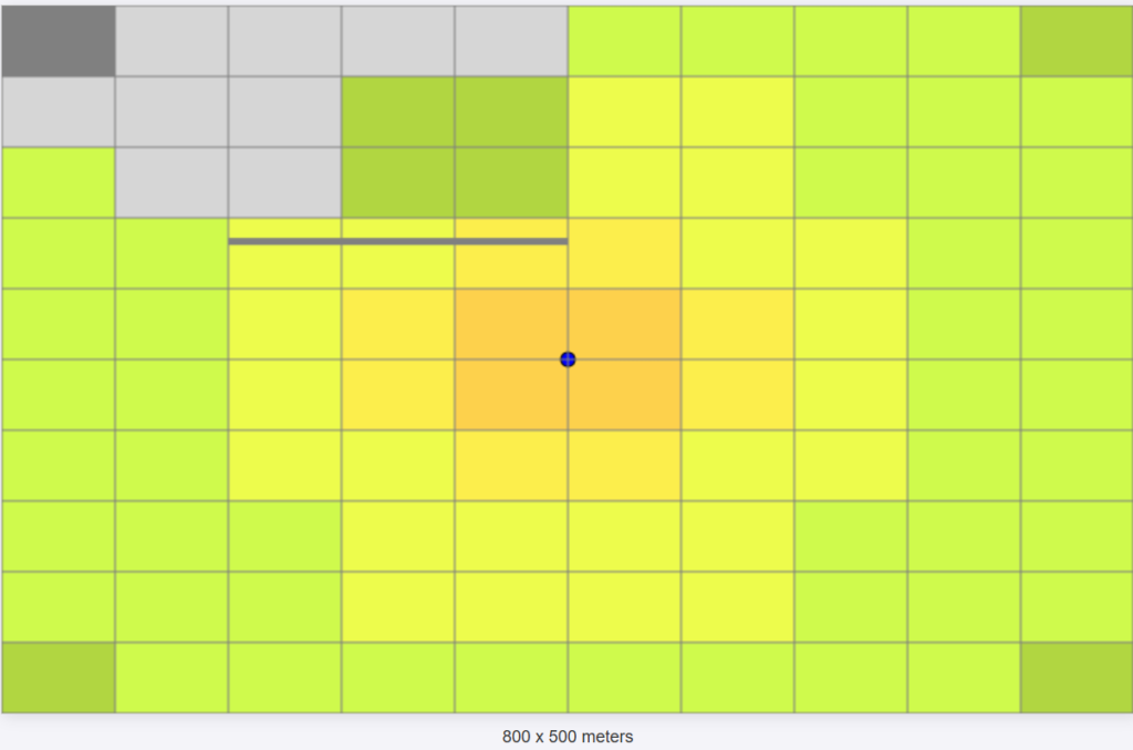
Great, it looks like it’s working as expected! Now, let’s check the RSSI before and after passing through the wall with an attenuation of 10 dB.

Now, let’s increase a little bit the number of blocks to improve the resolution of the image.

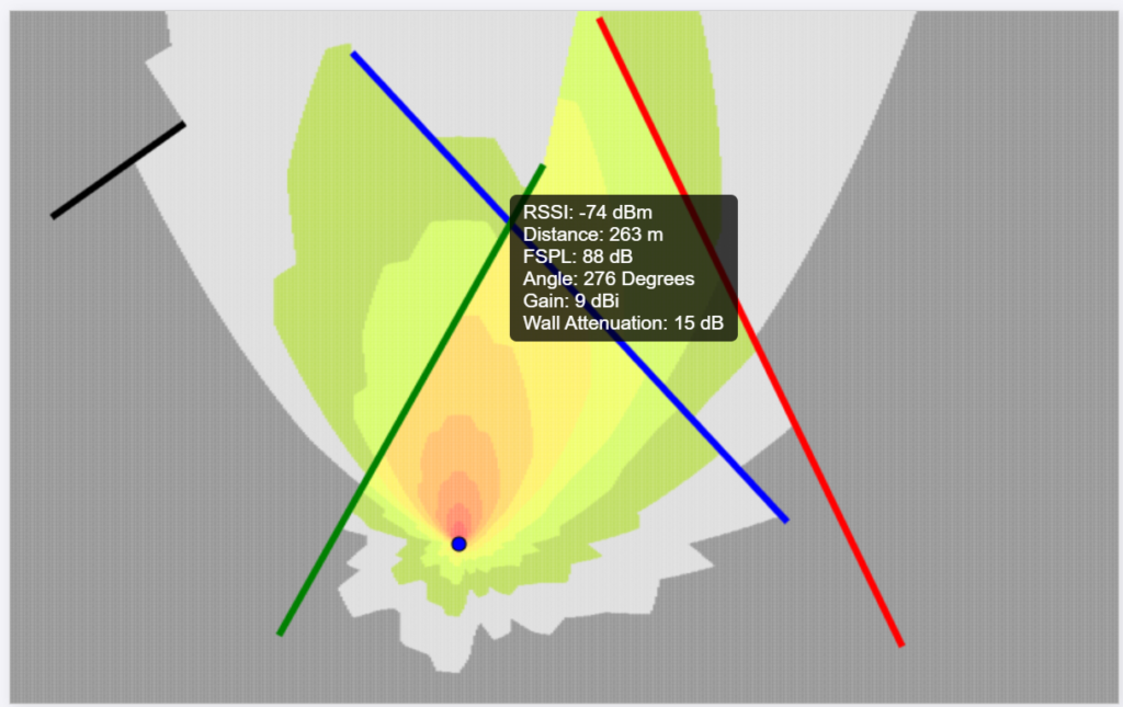
We can clearly see the effect caused by the wall attenuation!

To make things more interesting, I will add more walls.

Now, instead of each block accounting for the attenuation of a single wall, it will need to sum the attenuation from all the walls.

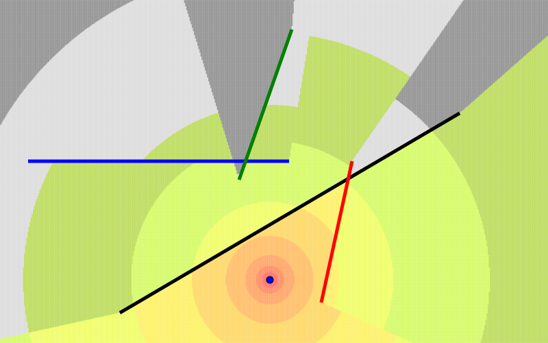
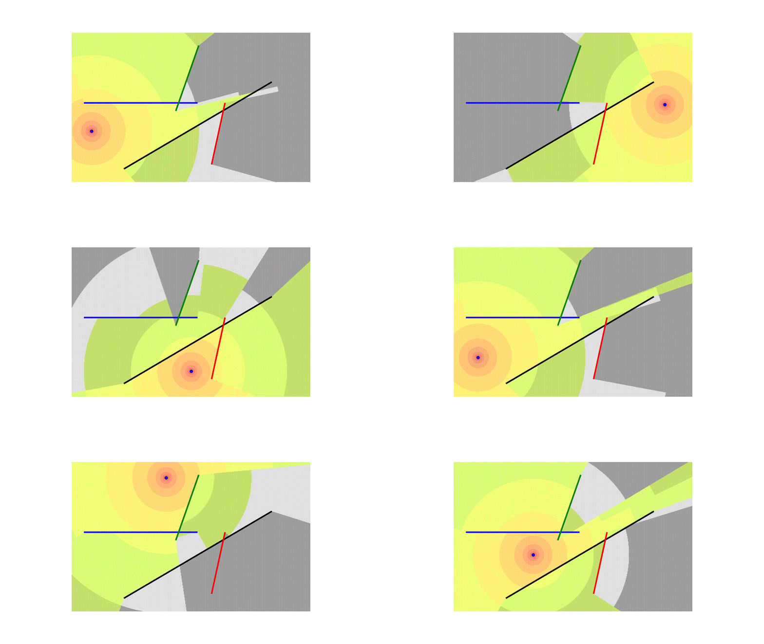
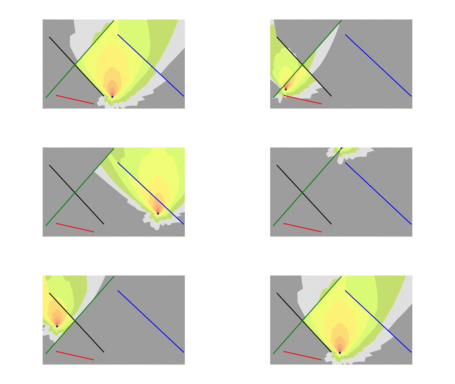
I also added the logic to handle special cases where the line segment from the transmitter to the center of the block is collinear with the walls and overlaps them.

These changes have been updated in my GitHub repository. Feel free to check it out!

https://github.com/dcapassi/js_simple_propagation_simulation

And that’s it! I hope you like it! Stay tuned for more!

Thanks

Diego Capassi