In my last post, I shared how I managed to grab some antenna data from Ekahau using a mouse clicker, a bit of Python, and a touch of creativity. It wasn’t the most sophisticated setup, but hey, it worked! The data lined up pretty well with what I expected, which was enough to keep me motivated.
This time, I decided to take it a step further and plug that data into the simple data visualization project I showed off earlier. Just to be clear, I’m not trying to build anything fancy or super useful for real-world decisions. This is more about experimenting, and showing how some basic math and scripting—plus a little curiosity—can open the door to the fascinating world of RF.
This should be a short post. (At least, that’s the plan!)
Quick Recap: From CSV to JSON
Last time, we exported a CSV file with gain and angle values for a specific antenna. I tweaked my script to spit out a JSON file instead, since JSON plays nice with JavaScript, which is what most simulation tools are built with these days.
Here’s what the JSON looks like:
[
    {
        "angle": 0,
        "gain": -15.57882772723093
    },
    {
        "angle": 5,
        "gain": -14.57882772723093
    },
    ...
]
This data comes from the Cisco 1562D antenna operating at 5GHz.
Using the Friis Equation
For this simulation, I’m working with the Friis transmission equation, which is all about calculating the received signal strength based on stuff like distance, frequency, and antenna gain.
Pr(dBm)=Pt(dBm)+Gt(dBi)+Gr(dBi)−FSPL
Where:
Pr: Power Received
Pt: Power Transmitted
Gt: Gain of the transmitter
Gt: Gain of the receiver
FSPL: Free Space Path Loss (20log10(d)−20log10(f)−20log10(c4π))
Previously, I left out the transmitter’s gain because it was set to zero. But now that we’ve got a proper list of gains mapped to angles, adding them into the mix is a lot easier.
The receiver’s gain will still be zero, since I have not collected the data of it.
How It Works
Here’s the plan:
- Figure out the angle
For every point in the simulation, determine its angle relative to the antenna. - Find the closest match
Since we probably won’t have an exact angle match in the data, we’ll use the nearest angle from the JSON file. - Adjust the signal strength
Add the gain from the JSON to the calculated signal strength. Keep in mind that gains can be negative, so this step can increase or decrease the signal strength.
Figure out the angle
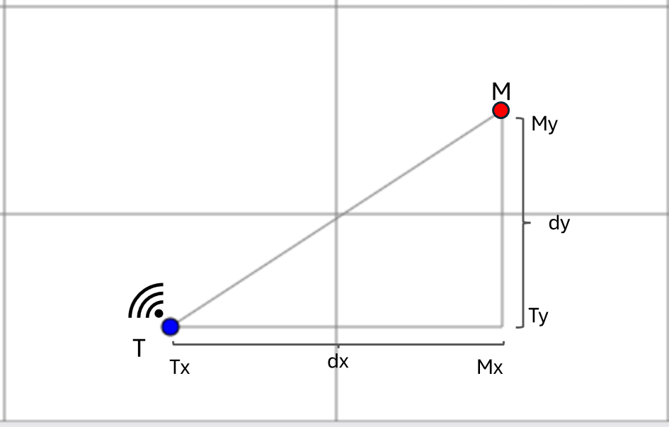
The first step is to calculate the angle between the center point of each block and the transmitter.

M is the measurement point, which is the center of the block, and T is the transmitter.
The angle can be found using the formula:
Angle (radians)=arctan(My−Ty, Myx−Tx)
To convert the angle to degrees, use the following formula:
Angle (degrees)=Angle (radians)×(π180)
The data was collected using 5-degree steps. If the point is 4 degrees away from the transmitter, no match will be found. To address this, the strategy is simple:
If no match is found, I interpolate the gain between the two nearest points (one lower and one higher in angle).
Formula:
y=y1+ ( (x−x1) / (x2−x1) )⋅(y2−y1)
Where:
x1 is the lower angle
y1 is the gain of lower angle
x2 is the upper angle
y2 is the gain fo the upper angle
y is the interpolated gain
Adjust the signal strength
This process is performed for each block, and now we can finally add the Gt (dBi) in the Friis equation:
Pr(dBm)=Pt(dBm)+Gt(dBi)−FSPL
Results

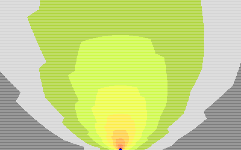
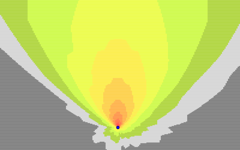
The results were quite good, and the interpolation helped make the visualization smoother. Below is the interpolation using a simpler approach, which calculates only the average between the upper and lower gain.

And that’s it! This isn’t about building the ultimate RF tool, but rather about demonstrating what’s possible with basic tools and a bit of curiosity. Of course, real modeling tools use a 3D approach for gain calculations.
I added this new feature to the simulation, repository: https://github.com/dcapassi/js_simple_propagation_simulation
Next, I’ll be adding some obstacles!
Thanks for following along—stay tuned.
Thanks,
Diego Capassi

